Usage
Image Annotating
Before start, prepare annotation data to train a classifier.
You should annotate at least two images; one for training and another for validating the model.
The annotation shape has to be rectangular. Since vodet uses the sliding-window method to detect the objects, very small sizes of rectangular relative to the size of the image will cause a very slow speed of detection. You should also make margins a little bit larger than the silhouettes of objects for better classification accuracy.
You can use either labelme or VoTT. Because labelme supports the zooming of images, I recommend you to use it, especially for high-resolution images.
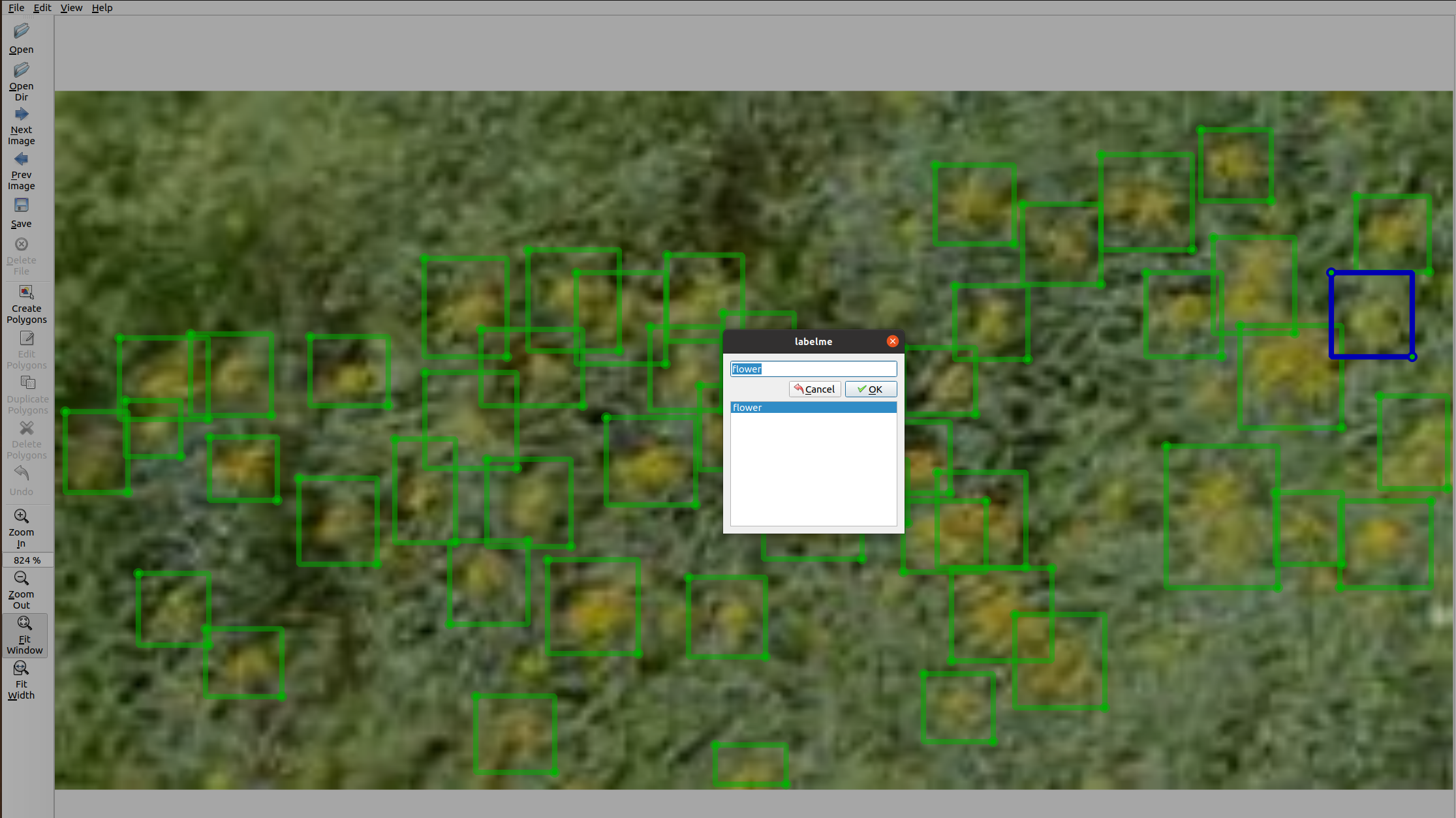 A screen shot of labelme’s user interface
Setting up data directories
The data directory should have three subdirectories: train, validation, and unlabelled.
The train and validation directory should have source and labels subdirectory, that contain source images and label data respectively.
The unlabelled directory should only have source directory.
The label data should be VoTT’s CSV-export (single CSV file) or labelme’s JSON files.
Notice:
All of the images you want to use in detection should be used in model training. Just push them all in the unlabelled directory, except for labeled images.
Directory structure example
.
├── train
│   ├── labels
│   │   └── IMAG0827.json
│   └── source
│       └── IMAG0827.JPG
├── unlabelled
│   └── source
│       ├── IMAG0417.JPG
│       ├── IMAG0441.JPG
│       ├── IMAG0463.JPG
│       ├── IMAG0485.JPG
.               .
.               .
.               .
│       └── IMAG1735.JPG
└── validation
    ├── labels
    │   └── IMAG0986.json
    └── source
        └── IMAG0986.JPG
Creating an GMVAE instance
from vodet.gmvae import GMVAE
data_dirs = {
    "train" : path_for_your_train_directory,
    "validation" : path_for_your_validation_directory,
    "unlabelled" : path_for_your_unlabelled_directory
}
gmvae = GMVAE(data_dirs)
for example,
from vodet.gmvae import GMVAE
data_dirs = {
    "train" : "./train/",
    "validation" : "./validation/,
    "unlabelled" : "./unlabelled/"
}
gmvae = GMVAE(data_dirs)
Generating patch images
To train the GMVAE classifier model, first, we separate source images into patches with labels based on label data.
With train and validation images, vodet read the label data created by annotation tools. A patch that intersects with rectangular annotations will be labeled as the label name (e.g. flower), otherwise others. With unlabelled images, sliding-windows crop images into patches. The patch sizes are randomly selected from that of train label data.
gmvae.set_patches("labelme") # for labelme
gmvae.set_patches("VoTT") # for VoTT
Then patches directory will be created inside the train, validation, unlabelled directory.
.
├── train
│   ├── labels
│   ├── patches
│   │   ├── flower
│   │   └── other
│   └── source
├── unlabelled
│   ├── patches
│   │   └── unlabelled
│   └── source
└── validation
    ├── labels
    ├── patches
    │   ├── flower
    │   └── other
    └── source
Preparing Dataloaders
Next, prepare torch.utils.dataloader with batch size and torchvision.transforms.
Important Notice
At least,
transforms.Resize((24,24))andtransforms.ToTensor()is required.The size of
transforms.Resize()must be (24,24).
from torchvision import transforms
transform = \
    {"labelled":transforms.Compose(
        [transforms.Resize((24,24)),
        transforms.RandomHorizontalFlip(),
        #transforms.ColorJitter(brightness=0.5,contrast=0.3),
        transforms.ToTensor()
        ]),
    "unlabelled":transforms.Compose(
        [transforms.Resize((24,24)),
        transforms.RandomHorizontalFlip(),
        transforms.ToTensor()
        ]),
    "validation":transforms.Compose(
        [transforms.Resize((24,24)),
        transforms.ToTensor()
        ])
    }

gmvae.set_dataloaders(batch_size=128, transforms=transform)
Model setting
gmvae.set_model(z_dim=8, device="cuda:0")
Then the model structure will be printed. For more details, please refer to the document of pixyz
Model:
Distributions (for training):
  p(x|z), q(z|x,y), p(y|x), p_{prior}(z|y)
Loss function:
  mean \left(- 32.0 \log p(y|x) \right) - mean \left(\mathbb{E}_{q(z,y_{u}|x_{u})} \left[\log p(z,x_{u}|y_{u}) - \log q(z,y_{u}|x_{u}) \right] \right) - mean \left(\mathbb{E}_{q(z|x,y)} \left[\log p(x,z|y) - \log q(z|x,y) \right] \right)
Optimizer:
  Adam (
  Parameter Group 0
      amsgrad: False
      betas: (0.9, 0.999)
      eps: 1e-08
      lr: 0.001
      weight_decay: 0
  )
Training
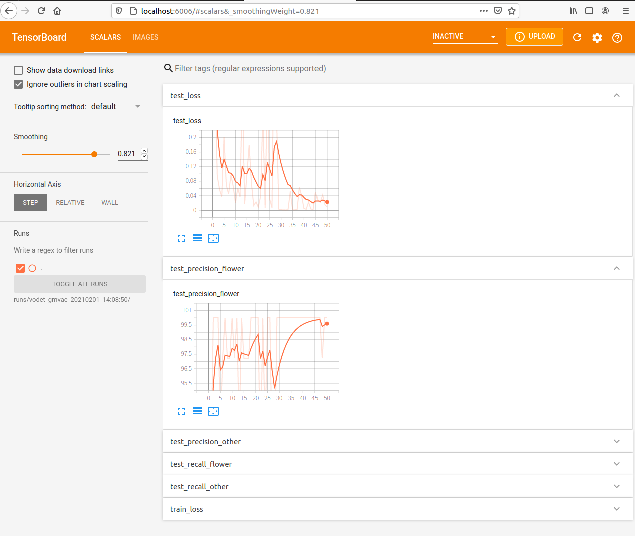
gmvae.train(epochs=50, precision_th=95.0)
While training, the GMVAE instance automatically saves the model parameters, as its attribute, with the lowest test loss. You can set the threshold of test precision to do this with precision_th.
Metrics of each epoch will be printed.
100%|███████████████████████████████████████████████████████████████████████████████████████████████████| 31/31 [00:01<00:00, 15.90it/s]
Epoch: 1 Train loss: 666.0989
Test Loss: tensor(0.3726, device='cuda:0') Test Recall: {'flower': 100.0, 'other': 90.0} Test Precision: {'flower': 89.74358974358974, 'other': 100.0}
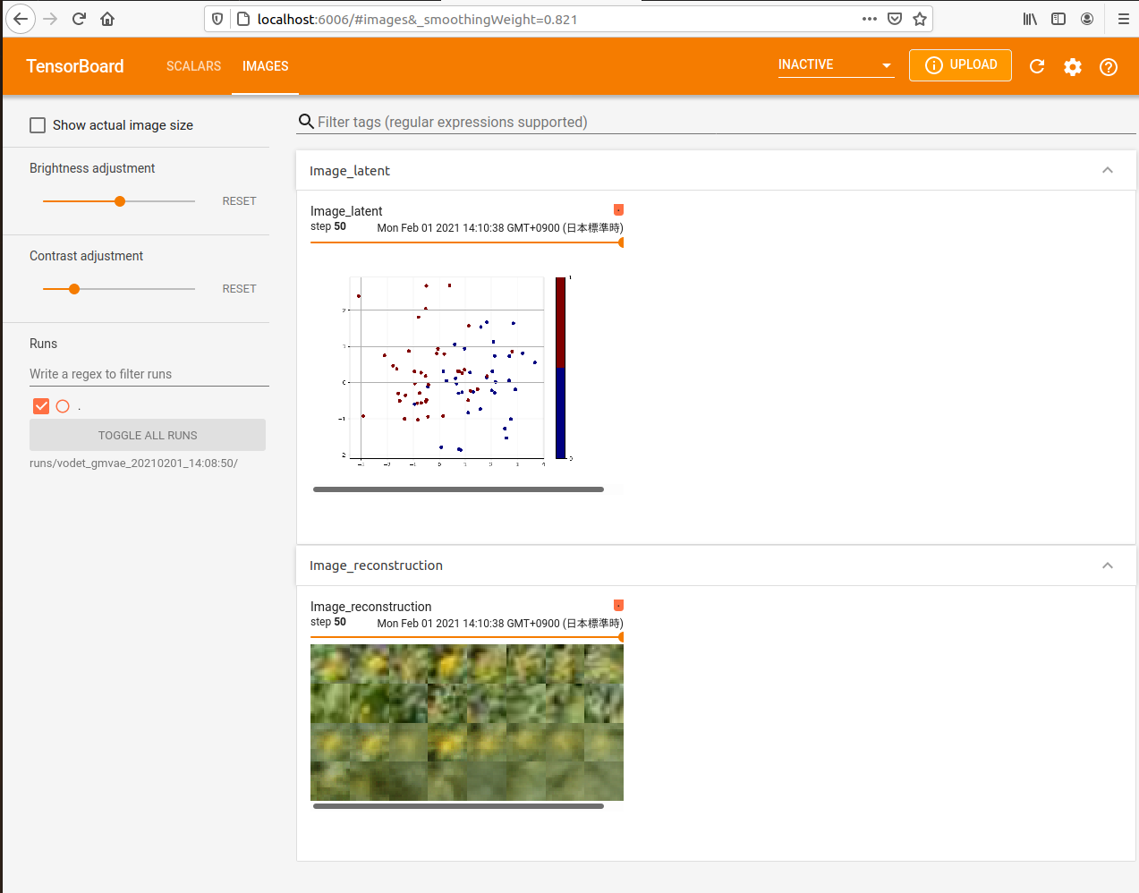
You can also inspect the training run with tensorboardX
The runs directory that contains the data of past runs as subdirectories will be created.
├── runs
│   └── vodet_gmvae_20210201_14:08:50
├── source
├── train
│   ├── labels
│   ├── patches
│   │   ├── flower
│   │   └── other
│   └── source
├── unlabelled
│   ├── patches
│   │   └── unlabelled
│   └── source
└── validation
    ├── labels
    ├── patches
    │   ├── flower
    │   └── other
    └── source
In this case, you can start tensorboard by running below in your terminal.
tensorboard --logdir runs/vodet_gmvae_20210201_14:08:50/
Detection
First, creat a classifier instance.
d = gmvae.detector(label_type="labelme", conf_th=0.99, step_ratio = 0.5, iou_th=0.05)
label_type: “labelme” or “VoTT”conf_th: Confidence threshold
step_ratio: The step size of sliding-windows relative to the size of them
iou_th: The threshold of Intersection over Union
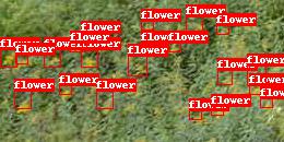
The detector object can perform detection for either single image or multiple images in a directory.
result_dict = d.detect_img("image_path", "out_path") # Single image
result_df = d.detect_dir("in_directory", "out_directory") # Multiple images in a directory
for example,
result_dict = d.detect_img("./test_data/test.jpg", "test_out.png") # Single image
result_df = d.detect_dir("./test_data/", "./test_out/") # Multiple images in a directory
Both of the function returns the object names and detected numbers, and also draw result image(s) in given path/directory.
Utility functions
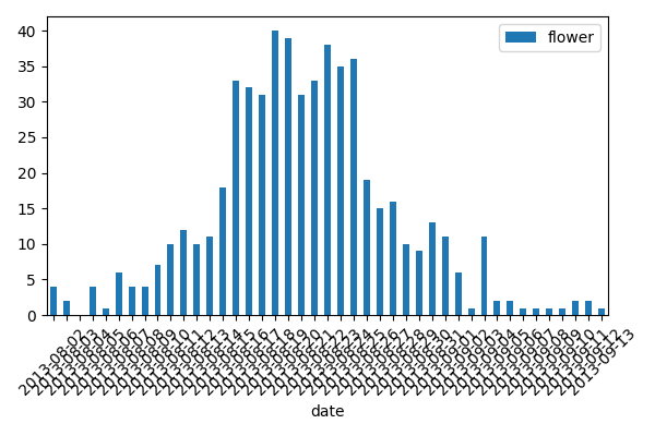
After running detection, you can plot detected results along time.
First, you should prepare a data frame with the image and date column that contains the file name and shooting date of each image. You can generate this automatically by using vodet.utils.exif_date() like below.
# Assume that the "source/" directory contains the original images with EXIF meta data.
from vodet.utils import date_df = exif_date("source/")
Then pass it to the detector instance.
resutl_df = d.draw_barplot(date_df)
Acknowledgements
All the example photographs of yellow flowers (Solidago gigantea) are taken at Tomakomai Flux Research Site in Tomakomai National Forest, Hokkaido, Japan, 2013 summer.